Fracture healing is steered by how the soft callus deforms, and walking deforms it differently at every instant. This page follows every integration point of one callus through a full gait cycle, classifies each point with a mechanobiological healing window, and then asks the same question of 278 fracture geometries.
0class mismatches, superposition vs direct run疊加法與直接計算的分類差異
Interactive bench
The callus, step by step骨痂,一步一步
Drag to rotate, scroll to zoom, double-click to fit, drag the timeline to scrub. Step through a series with ◀ ▶. Every point is recomputed live from the three unit-load solutions. The cards on the right walk through the story.
Each dot is one of the 33,712 integration points of the reference callus (wedge 0°). The knee force at 1 km/h, scaled to 70 %, is applied in 101 steps. Colour is the tissue the selected healing window predicts for that point.
每個點是參考骨痂(楔形 0°)33,712 個積分點之一。1 km/h 的膝關節力乘以 0.7,分 101 步施加。顏色是所選癒合窗為該點預測的組織。
Cycle-mean volume fractions · 週期平均體積分率
02 · why the whole cycle
The load peak is not the average峰值載荷不等於平均
At the force peak (gait 0 %) only 49 % of the callus is in the bone zone; averaged over the whole cycle it is 79 %, because most of the cycle is low load. The moment you evaluate changes the answer: Claes & Heigele (1999) and Simon (2011) calibrated their windows at peak load.
The strain plane (top right) shows volumetric strain against octahedral shear strain. The background is coloured by tissue (bone, cartilage, connective tissue, destructive); each white dot is one point of the callus. The plane shows the boundary chosen in the Window menu: the Simon rectangle (solid line) or the ellipse (dashed line), with the background coloured by that boundary's regions. Switch between the two to see which points change tissue. The Scale window limits slider scales every limit.
Only a narrow fan of the window is used癒合窗只有一個窄扇形被用到
A soft layer between stiff fragments is pushed and pulled almost in one direction only, so each point slides back and forth along a straight line in the strain plane. Poisson's ratio fixes the angle of that line (about 79° and 101° for a ratio of 0.167). Across all 278 models, 90 % of the exposure lies between about 72° and 104°.
Live: how much callus volume and time falls at each direction angle; dashed lines mark the two straight-line directions · 即時:各方向角度上累積的骨痂體積與時間;虛線標出兩條直線方向
05 · cycle summary
Time spent in the bone zone停留在成骨區的時間
Set Colour to “Cycle: time in Bone zone”. A point that is bone on average can still spend a third of the cycle in cartilage or connective stimulus. Rotate the cloud to see where those points are.
把「Colour」設為 “Cycle: time in Bone zone”。平均看起來是「骨」的點,仍可能有三分之一的時間處於軟骨或結締組織刺激。旋轉點雲看看這些點在哪裡。
06 · weight bearing
Load fraction moves the window負重比例會移動癒合窗結果
The Load slider sets the fraction of the healthy-subject force (50–100 %). The solve is linear, so every point is reclassified live. This card uses 100 %; above 70 % the callus rotates beyond the range the linear analysis was validated for, so treat it as illustration.
The validated speeds (1, 1.5 and 2 km/h) differ mainly in the shape of the load history, not its peak (2.07–2.38 kN). Faster speeds can be selected in the Speed menu but are outside the linear range: illustration only.
In the Model row pick a series (grouped by family), then step with ◀ ▶ or the arrow keys, or press Play models to sweep the series back and forth. Only the model changes: gait step, window, speed, load, colour and view stay. With same scale on, one camera scale is shared so the growth of the callus is visible. This card loads wedge 65°. For all 17 model types side by side, see chart 1 of Sweep.
在「Model」列選一個系列(依家族分組),用 ◀ ▶ 或鍵盤方向鍵一步一步換,或按 Play models 讓系列來回自動播放。只有模型改變:步態、癒合窗、步速、負重、顏色和視角都不動。勾選 same scale 時整個系列共用同一個相機比例,骨痂的大小變化看得出來。此卡片載入楔形 65°。想把 17 種模型類型並排比較,請看「Sweep」的圖 1。
09 · other windows
Same callus, another window同一個骨痂,不同的癒合窗
A healing window is two independent choices, so the table is a grid. Coordinates (the three groups) are how volume change and distortion are computed for each point: from the small strain; from the principal stretches (Version B, V and D, rigid rotation ignored); or from the full deformation gradient (rigid rotation counts as deformation). Boundary (the two rows in each group) is the Simon rectangle or the ellipse with the same limits (bone 0.85 % × 7 %, outer 5 % × 16 %), see The healing window. Claes M0 has other, asymmetric limits and is listed apart as a reference.
Two numbers answer two questions. Difference (third row of each group): how much of the callus the two boundaries classify differently in the same coordinates, the effect of the shape. vs small strain: how much the same boundary changes when the coordinates change, the effect of the coordinates. Click a row to show it on the cloud: Rectangle, Ellipse, or Difference, which keeps only the points the two classify differently.
癒合窗有兩個互相獨立的選擇,所以表格排成格子。座標(三個群組)是每個點的體積變化與畸變怎麼算:用小應變;用主伸長(Version B 的 V 與 D,忽略剛體旋轉);或用完整的變形梯度(剛體旋轉也算成變形)。邊界(每組的兩列)是 Simon 矩形,或界線相同的橢圓(骨 0.85 % × 7 %,外圈 5 % × 16 %),見「癒合窗」一節。Claes M0 的界線不同而且不對稱,單獨列在最後當參考。
兩個數字回答兩個問題。Difference(每組的第三列):同一組座標下,兩種邊界分類不同的骨痂比例,也就是形狀的影響。vs small strain:同一種邊界換了座標後分類改變的比例,也就是座標的影響。點選任一列即可在點雲上顯示:Rectangle、Ellipse,或 Difference(只留下兩者分類不同的點)。
Three views per coordinate system: click Rectangle, Ellipse or Difference. Difference shows only the part of the callus the two boundaries classify differently; its bar is the make-up of that part by the ellipse's tissue. All percentages are shares of the callus volume.
The healing window
From strain space to finite-deformation invariants從應變空間到有限變形不變量
The bench above sorts every point of the callus with a healing window. This section explains that window: where its boundary comes from, why an ellipse is worth testing against the usual rectangle, how both boundaries are carried from strain space into finite-deformation invariants, and what the two look like when drawn together on the same axes.
Claes and Heigele established the threshold-window logic that links local mechanics to tissue outcome: below some strain and hydrostatic limits a point forms bone, in a wider band cartilage or connective tissue, and beyond that it is destructive. Later models changed the mechanical coordinates and the biological rules but kept the idea of a window.
This study uses the symmetric dilatational–distortional version, so that the two boundary shapes can be compared under identical conditions.
本研究採用對稱的「體積–畸變」版本,好讓兩種邊界形狀能在完全相同的條件下比較。
Bone window
\(|v|\le 0.85\,\%,\ \ s\le 7\,\%\)
Inner threshold: bone formation.
內層閾值:成骨。
Outer window
\(|v|\le 5\,\%,\ \ s\le 16\,\%\)
Cartilage on the compressive side (\(v\lt -0.85\,\%\)), connective tissue elsewhere; outside is destructive.
壓縮側(\(v\lt -0.85\,\%\))為軟骨,其餘為結締組織;超出則破壞。
\(v\) = volumetric (hydrostatic) strain, \(s\) = octahedral shear strain, \(s\ge 0\). The Claes thresholds are anchors; the symmetric version is a study choice, not a claim about Claes.
Why introduce an ellipse, and how is it constructed?為什麼要引入橢圓?怎麼構造?
A rectangle treats volume and shear as independent: a point is accepted if \(|v|\) and \(s\) each stay under their own limit. That gives sharp corners. A point at the corner of the bone box, with the largest allowed volume change and the largest allowed shear at the same time, passes, even though it is the most demanding state in the box. An ellipse couples the two: the more volume change a point has, the less shear it is allowed.
The ellipse passes through the same axis intercepts as the rectangle, so the two differ only in how they cut the corners.
橢圓與矩形有相同的軸截距,所以兩者只差在「怎麼切掉角落」。
The ellipse is introduced as an \(L_p\)-sensitivity hypothesis, not as an established Claes-family boundary. The cartilage / connective split on the ellipse is a ray at \(\varphi=99.8^{\circ}\); it ends on the outer ellipse exactly at \(v=-0.85\,\%\), the same \(v\) where the rectangle separates cartilage from connective tissue.
A window defined on \((v,\,s)\) is a statement about strain. To use it with a finite-deformation solver it has to be restated through the deformation itself. The chain below follows the 0610 whiteboard derivation; every later figure is generated from it.
To draw the finite panels, each \((v,\,s)\) is sent to principal stretches along an axisymmetric path that preserves \(v\) and \(s\), then through the chain above:
Both windows are defined on the same \((v,\,s)\) plane with the same anchors. So in every projection they are the same boundary curves pushed through the same map, and can be drawn on one set of axes without approximation. Shading follows the ellipse; the rectangle is laid over it.
All six panels are drawn live in your browser from the formulas on this page. Lines are coloured by tissue: gold for the outer window, green for the bone window, blue for the cartilage divider; the switch above tints the regions as well. Hover a panel to read the strain, and what each window says about that same point. The raw finite invariant plane \((\mathrm{III}_C,\mathrm{II}_C)\) is left out: both windows collapse into one thin diagonal band there, so it carries no information about the boundary shape. It is kept only as a diagnostic control.
The ellipse lies inside the rectangle and touches it only at the axis intercepts. Everything in the four corners, such as \(|v|=5\,\%\) together with \(s=16\,\%\), is accepted by the rectangle and rejected by the ellipse.
Linearising \(\det(\mathbf I+\nabla\mathbf u)\) and splitting \(\boldsymbol\varepsilon=v\,\mathbf I+\boldsymbol\varepsilon\,{}^{\prime}\) turns the strain plane into a parabola-shaped region. The raw \(\mathrm{II}\) still carries a volume term.
Removing the volume factor separates the two roles, but the coordinates are not centred: the undeformed state sits at (1, 3), not at the origin.
扣除體積因子後,兩個角色分開了,但座標沒有置中:未變形狀態在 (1, 3),不在原點。
What to look at看什麼
The rectangle's top edge is no longer horizontal: the map is non-linear, so a constant shear limit tilts with volume. The ellipse stays a smooth dome inside it.
矩形的上緣不再水平:映射是非線性的,恆定的剪切上限會隨體積傾斜。橢圓仍是它裡面一個平滑的圓頂。
E · Finite, Version C
\((J,\mathrm{II}_{\bar C})\): the Jacobian as volume axis\((J,\mathrm{II}_{\bar C})\):以 Jacobian 為體積軸
Taking the positive square root gives a volume axis with a direct physical meaning, \(J\) = deformed volume ÷ original volume. The distortion axis is unchanged.
取正的平方根,得到一條有直接物理意義的體積軸,\(J\)=變形後體積 ÷ 原體積;畸變軸不變。
F · Finite, Version B
\((V,\,D)\): centred, directly comparable with Claes\((V,\,D)\):置中,可直接對照 Claes
Centring puts the undeformed state at the origin and makes the axes mean the same thing as the Claes strains, so this is the plane most directly comparable with panel A.
置中後,未變形狀態在原點,座標軸的意義與 Claes 應變一致,所以這是與圖 A 最能直接對照的平面。
What to look at看什麼
The picture is panel A again with a slight shear bend: the rectangle's side edges lean and its top edge slopes, while the ellipse stays inside. The ordering, ellipse within rectangle, survives the finite map.
這張圖就是圖 A 加上輕微的剪切彎曲:矩形的側邊微斜、頂邊傾斜,橢圓仍在裡面。「橢圓在矩形之內」這個次序在有限變形映射下保持不變。
05 · Status
What is established and what is open已確認與尚未確認
Completed
Consistent small- and finite-deformation derivation小變形與有限變形推導一致
Three finite coordinate versions (A, B, C)三種有限變形座標(A、B、C)
Mechanics mapping checked on canonical paths: simple shear, pure shear, pure dilation, shear with volume change力學映射已在典型路徑上驗證:簡單剪切、純剪切、純膨脹、剪切疊加體積變化
Current limits
Finite panels use an axisymmetric proxy有限變形的圖用軸對稱代理路徑
They are 2D mechanics projections, not exact Gauss-point states它們是二維力學投影,不是精確的高斯點狀態
The ellipse is a sensitivity hypothesis; the biological boundary is not established橢圓是敏感度假設;生物學邊界尚未確立
Next simulation step
Export \(\mathbf F\), \(\mathbf C\) or true principal stretches from the solver從求解器輸出 \(\mathbf F\)、\(\mathbf C\) 或真實主伸長
Compute \(J\), \(\mathbf C\), \(\mathrm{II}_{\bar C}\), \(V\) and \(D\) per integration point逐積分點計算 \(J\)、\(\mathbf C\)、\(\mathrm{II}_{\bar C}\)、\(V\)、\(D\)
Overlay the point cloud on these merged planes, then test sensitivity to the boundary shape把點雲疊到這些合併平面上,再檢驗對邊界形狀的敏感度
Current claim: the mechanics mapping is verified on canonical paths; the biological boundaries and real Gauss-point overlays remain open.
目前的主張:力學映射已在典型路徑上驗證;生物學邊界與真實高斯點疊圖仍待完成。
The model
A nailed tibia, 278 ways to break it一根打了髓內釘的脛骨,278 種斷法
Every model is a bare tibia with an intramedullary nail and a callus generated from the fracture gap. All materials are linear elastic and there is no contact. The ankle end is fixed; the gait force is split evenly over the 1,907 nodes of the tibial plateau, which is otherwise free.
The fibula is left out on purpose. The large plateau displacement is a consequence of that choice, not a modelling error; models with a fibula are a separate, later study.
腓骨是刻意不放的。平台位移大是這個選擇的結果,不是建模錯誤;含腓骨的模型是之後另一個研究。
The force is the knee joint contact force from Xsens motion capture through a musculoskeletal model, so muscle forces are included. That is why it peaks at several times body weight.
341,715 nodes · 236,253 C3D10 elements per mesh (reference model). The four fracture families and their parameters are listed in Sweep.每個網格 341,715 節點、236,253 個 C3D10 元素(參考模型)。四個骨折家族與它們的參數列在「Sweep」一節。
Pipeline
Solve three times, walk any cycle只解三次,就能走任何週期
Because the analysis is linear and the load pattern is fixed, every field at every instant is a weighted sum of three unit-load solutions. One 50-second job per model replaces 101 separate steps, and speed, weight bearing and step count become post-processing.
u(t) = Fx(t)·ux + Fy(t)·uy + Fz(t)·uzsame for ε, σ and F − I · ε、σ、F − I 同理
BuildAppend 3 unit steps (1 kN in x, y, z) to the mesh; nail set to 108,000 MPa.在網格後加三個單位載荷步(x、y、z 各 1 kN)。1–2 s
SolveAbaqus, one matrix decomposition, 6 jobs × 4 cores in parallel.Abaqus 只分解一次矩陣,6 個 4 核工作並行。≈ 50 s / model
Extract104 columns per integration point, including det F from nodal displacements.每個積分點 104 欄,含由節點位移算出的 det F。≈ 4 s
SuperposeAny force history × 0.7, rolled so the peak is at 0 %: 3 speeds × 101 steps.任意力歷程 × 0.7,峰值對齊 0 %:3 種步速 × 101 步。≈ 40 s / model
Classify + QASimon (primary) and Claes M0 windows; equilibrium, shape functions, det F > 0 gates.Simon(主)與 Claes M0 癒合窗;平衡、形函數、det F > 0 檢查。seconds
The full sweep ran 278 models × 3 speeds = 834 scenario rows in 138 minutes of wall time. With the calibrated force direction (October 2026), 275 models pass every gate; 3 spiral models are flagged because a tiny part of their callus (≤ 0.002 %) inverts. The bench above repeats steps 4 and 5 in your browser and reproduces the sweep index for the reference model to 1e-16.
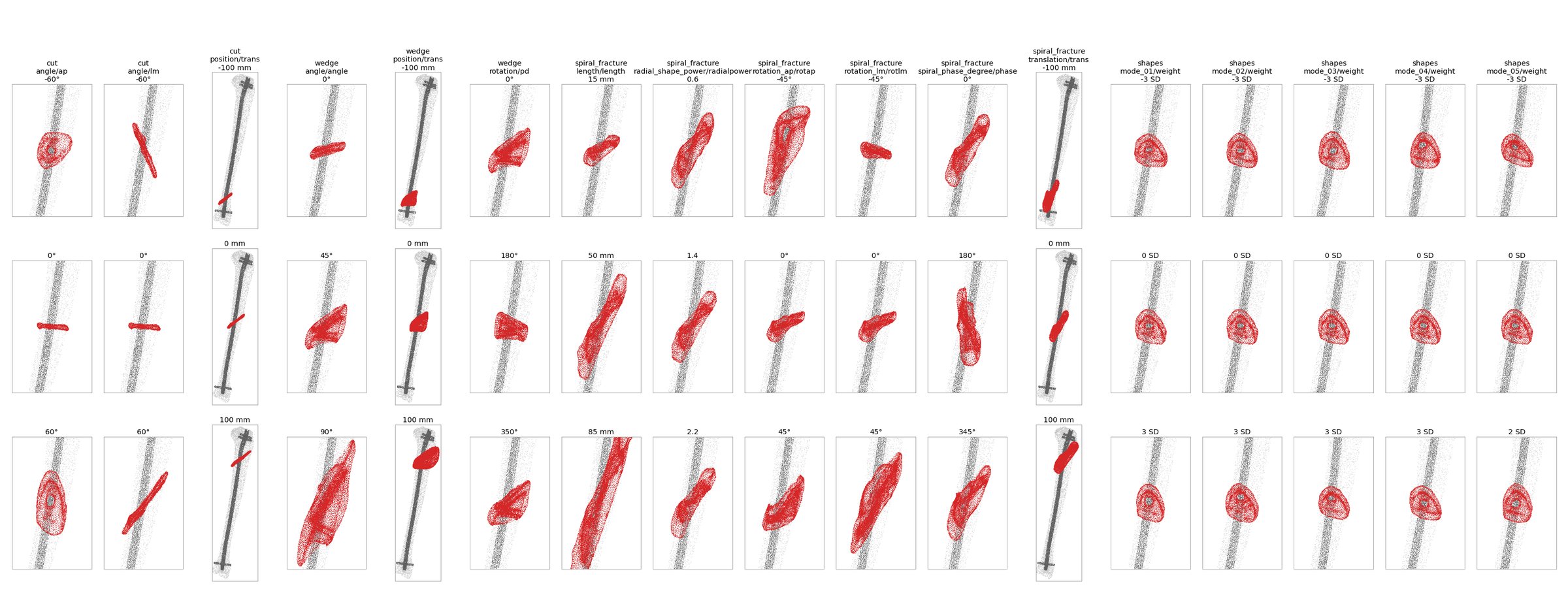
Every mesh belongs to one model type: a fracture family (cut, wedge, spiral, shapes) with one varied parameter, 17 types in all. Choose a metric and a speed once in the bar below. The charts then show that metric three ways: along the parameter of each type, over the force of the gait cycle, and against callus volume.
278 files hold 269 distinct geometries, and the series do not share one baseline.278 個檔案實際是 269 種不同幾何,各系列的基準也不相同。
Callus (red) on the tibia and nail for every series at its lowest, zero and highest parameter value. Scroll sideways.每個系列在參數最小、零與最大值時的骨痂(紅色)。可左右捲動。
1 · Along the parameter of each model type
One chart per model type; the x-axis is the varied parameter. Tissue is split into two groups: bone + cartilage, the positive stimulus (blue), and the rest, that is connective, resorption and destructive (orange). Δ is the highest minus the lowest value along the parameter. Click a dot to load that model in the bench; click a title to open the type in chart 2.
The force sweep is the gait cycle itself: 101 steps, each with its own force. Every line is one model of the chosen type; each of its 101 steps sits at the force of that step (x) and the share of callus volume in the bone or cartilage zone at that step (y). This chart always shows bone + cartilage; the speed follows the bar above. Colour is the value of the varied parameter. Cycle Δ is the highest minus the lowest share within one cycle, averaged over the models of the type. Hover a line for the model, click to load it in the bench at that step.
Each dot is one mesh; hover for its name, click to load it. The callus is generated from the fracture gap and its size varies tenfold. Callus size explains a large part of the between-type spread in bone + cartilage (r shown above for the visible set). Larger calluses spread the same load over more tissue, so they look more bone-like even when the gap moves more. Fracture types therefore have to be compared alongside volume, or volume-normalised.
Each bar is one model: the 5th to 95th percentile of θ over the whole cycle, dot at the median, sorted by median. No model leaves the band 69.4°–108.0°. The two dashed lines are the uniaxial rays for ν = 0.167.
Accepted on the reference model, where 2.4 % of the callus rotates more than 10°. Across the sweep (calibrated force), 43 models exceed 10 % of the callus and 3 exceed 25 %. Rankings within a series are safe; absolute fractions above 25 % need NLGEOM checks.
Simon's thresholds were calibrated with a 3 MPa, ν = 0.30 callus; these models use 1 MPa, ν = 0.167. The choice of window moves Resorption by 0.06, more than the strain measure does. Cartilage and Connective fractions are for ranking only.
Different meshes (parametric wedge vs the FKA patient tibia), so the comparison is behavioural. Both put the resorption spike at 20–40 % of gait, where Fz passes through zero, and both are bone-dominated under load.
網格不同(參數化楔形 vs FKA 病人脛骨),因此比的是行為。兩者都把吸收高峰放在步態 20–40 %(Fz 過零處),且在受載時都以骨為主。
Next
Open questions待解問題
Ordered by how much each would change the argument.
依對論證影響大小排序。
Evaluate where the window was calibrated. Peak load (or a high percentile), in the gap and on the bony surfaces, with an absolute or bridging indicator instead of the whole-callus fraction.在癒合窗校準的條件下評估:峰值載荷(或高百分位)、間隙與骨表面,並使用絕對量或橋接指標,而非全骨痂比例。
NLGEOM sensitivity on the ten most rotated models plus wedge/position trans_0 and spiral/translation trans_0.對旋轉最大的十個模型加上 wedge/position trans_0 與 spiral/translation trans_0 做 NLGEOM 敏感度分析。
Calibration material run: callus 3 MPa, ν = 0.30, one 50-second unit job.校準材料計算:骨痂 3 MPa、ν = 0.30,一個 50 秒的單位載荷計算。
Cycle variability: use all 6–13 measured cycles per speed so each window becomes a distribution.週期變異:每種步速用全部 6–13 個量測週期,讓每個結果變成分布。
Load frame: done (October 2026). The knee force is now applied in the anatomical frame of each mesh: long axis along the nail, antero-posterior and medio-lateral components no longer swapped. All results on this page use it.載荷座標:已完成(2026 年 10 月)。膝關節力改為加在每個網格的解剖座標:長軸分量沿髓內釘,前後與內外分量不再對調。本頁所有結果都用校準後的力。